Project Management Info Can Be Found On Our Website!
Background
Fundus images require careful analysis, but literature suggests that AI is feasible here. A survey of AI approaches to diabetic retinopathy remarked: “artificial intelligence models are among the most promising solutions to tackle the burden of diabetic retinopathy management in a comprehensive manner” \(^{[1]}\). A survey of AI age-related macular degeneration models concluded: “the application of AI-based automatic tools is beneficial for the diagnosis of AMD” \(^{[2]}\). Finally, a survey of AI glaucoma diagnosis models stated: “computerised image processing technologies … are time-efficient, reproducible and often more accurate than human experts” \(^{[3]}\). In all of these disparate cases, AI proved to be diagnostically relevant!
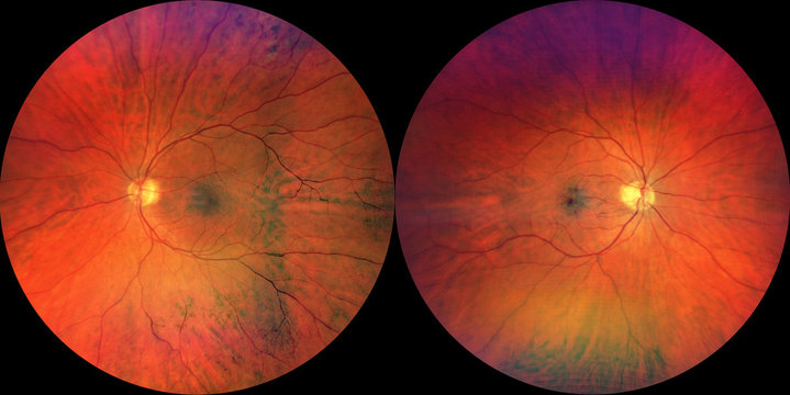
We identified a dataset containing thousands of colored fundus images prelabeled with the associated pathology (or lack thereof). Initially, we will focus solely on macular degeneration, though as we progress we may include more classes in our models and analysis.
Problem Definition
Ophthalmic (eye) diseases are often debilitating and irreversible, affecting the vision of millions of people across the world. Diagnostic tools for these diseases do exist, but they can be costly and often rely on the diagnostician’s discretion, leaving room for error. Thus, there exists a demand for a tool to aid in diagnosis.
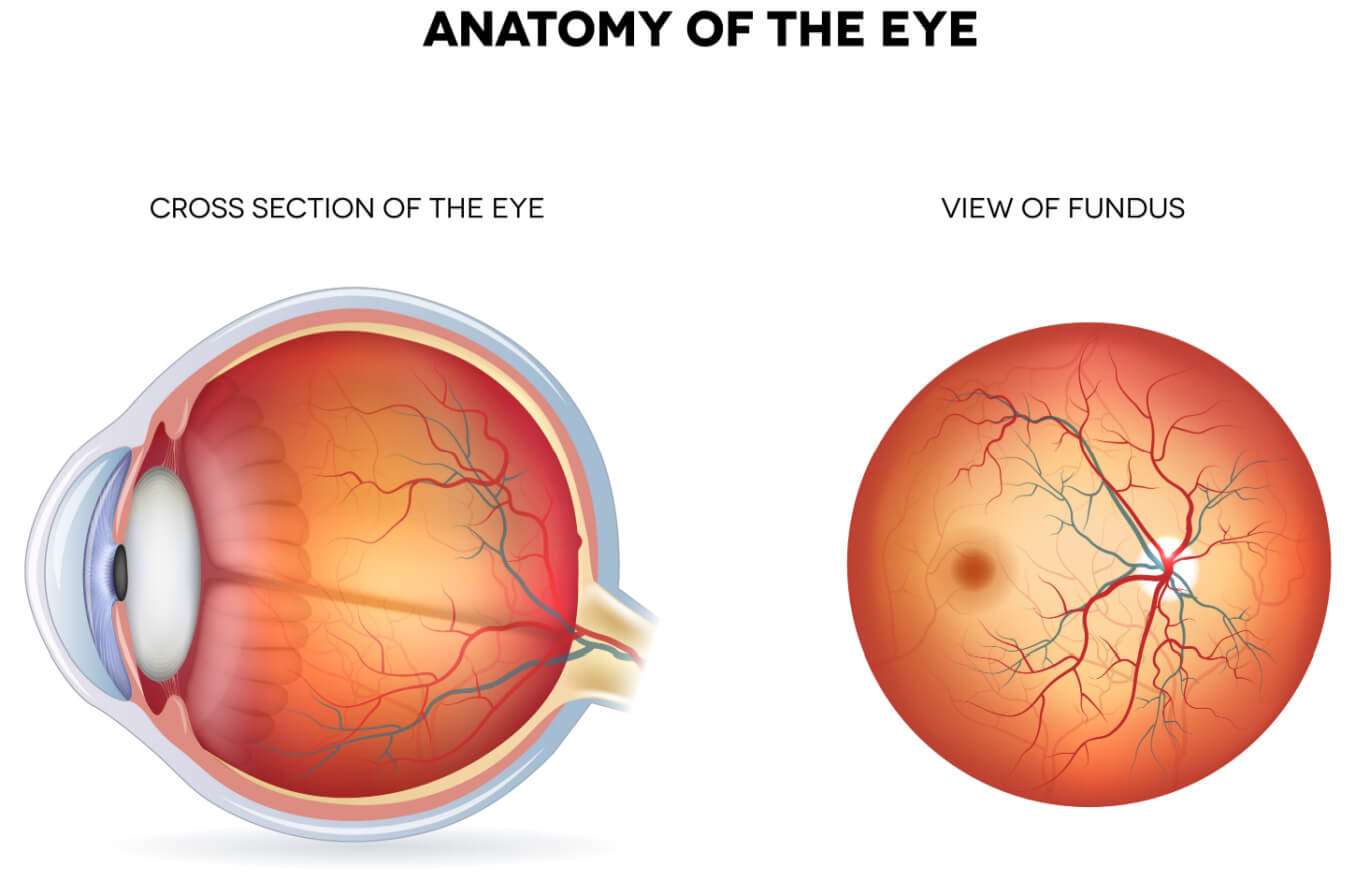
One potential solution is AI fundus image analysis. A fundus image is a capture of the retina from a relatively cheap and non-invasive camera, offering scalable and equitable access. Many pathologies are diagnosable from irregularities in fundus images. Thus, we want to test the feasibility of AI diagnosis using fundus images.
Model #1: SVM
The first model we attempted is called Support Vector Machine (SVM), which is a supervised learning technique. SVMs simply fit for the maximum-margin linear surface that classifies the largest part of the training space correctly \(^{[4]}\).
We chose SVM because we wanted to implement a naive supervised learning technique before moving on to more complex neural networks. Additionally, SVM has the benefit of sustained performance in very high dimensionality data, which fits our purpose, since our input is images.

This is an example of SVM on a 2D dataset
Feature Extraction
We also utilized a feature extraction technique called the Histogram of Oriented Gradients Descriptor (HOG). HOG partitions the image into cells, calculates the pixel gradient for each cell, then arranges those gradient vectors into bins, and places them on a histogram. By aggregating pixel information into descriptors, the dimensionality of image-based input can be drastically reduced \(^{[5]}\). Below is an example of what it looks like on a sample image.
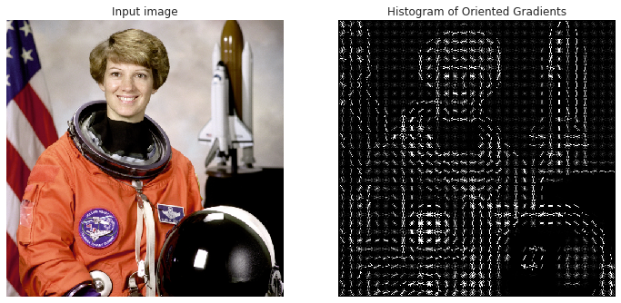
We used this method because of knowledge about the problem space. A fundus image of a healthy retina tends to be relatively smooth and uniform, save for veins and arteries, while afflictions like diabetic retinopathy can create visible deformities, like fatty exudates or hemorrhages, which causes, on average, a distinctly higher pixel gradient.

Example run of HOG on two zoomed in portions of training images
Our pipeline is as follows:
- Resize the image to 700x1050 (since different cameras in the dataset have different aspect ratios)
- Convert the image to grayscale (since different cameras have different color interpretations)
- Convert the image to a HOG descriptor vector using 16p x 16p cells (to achieve feature reduction)
- Train the SVM using class weights and a radial basis kernel function (to capture potential non-linear relationships)
Results
Running SVM on the images alone

- Accuracy: 74.74%
- f1-Measure: [0.4641, 0.83475]
- Diagnostic Odds Ratio: 4.455
Running SVM with image processing
- Accuracy: 84.90%
- f1-Measure: [0.6234, 0.9055]
- Diagnostic Odds Ratio: 16.04
Analysis of Results
After our optimizations, the model clearly performs much better. The accuracy and f1-measures are much higher and meet our targets from our original proposal. The diagnostic odds ratio is 4 times higher, so as a diagnostic tool, the test is 4 times more informative. This is below our target for DOR, since the model is not as effective at predicting healthy retinas as it is at predicting unhealthy retinas, but it is still an improvement.
Next Steps
By doing more rigorous cross-validation, the performance of this model could likely improve.
Model #2: Neural Network
We developed a Neural Network as the second machine-learning algorithm. We chose this model because properly tuned neural networks can be very accurate while requiring minimal data preprocessing relative to other machine learning techniques.
We began with a Multi-Layer Perceptron (MLP) Classifier from Scikit learn as our neural network, and kept the network relatively shallow for performance reasons. We had 2 layers with 15 and 7 neutrons respectively. However, as we tuned the model, we did not find any significant increase in performance by making it deeper.
Prior to feeding the images into the MLP Classifier for training, we cropped the images to a 500x500 square. This allowed for a significant decrease in the size of the image (about 4x smaller) while still keeping the majority of the information. This cropping keeps the input to the model smaller, increasing the speed of the model.
Despite our best efforts, we were unable to reach the performance we were expecting with Scikit’s MLP classifier, so we made the switch to a PyTorch Convolutional Neural Network. Our first network architecture consisted of 4 convolutional layers, followed by three linear layers and a sigmoid output for binary classification between healthy and unhealthy eyes.
Initial Neural Network Schematic:

Our initial network failed to meet our expected performance, despite various tuning techniques, so we made a change to our architecture. These changes included removing a convolutional layer, making one of the convolutional layers a 7x7 compared to the previous 3x3, removing dropout layers, adding more max pooling layers, removing a linear classification later, and adding batch normalization to increase network consistency.
Final Neural Network Schematic:

Results
Intial Tuning
After our first attempt at tuning the neural network, the model was achieving an accuracy of 79.06%, however, on inspection of the results, the neural network predicted that all of the images were at risk for disease due to the bias in the dataset. The statistics of this version of the model can be seen below. After brainstorming some potential solutions to this issue, we settled on using a weighted loss function to fix it. While this is not supported by Scikit learn’s MLP Classifier, it is supported by PyTorch neural networks \(^{[6]}\). This was one of our motivating factors behind why we would later switch to PyTorch.

- Accuracy: 79.06%
- f1-Measure: [0, 0.8831]
- Diagnostic Odds Ratio: NAN
Neuron Decrease Breakthrough
After a bit more tuning, we found that decreasing the neurons in our neural network layers from 20 and 10 to 15 and 7 significantly improved the performance of the model. We achieved 84.38% accuracy, with the model making a true attempt at predicting based on the images.
- Accuracy: 84.38%
- f1-Measure: [0.4505, 0.9089]
- Diagnostic Odds Ratio: 41.43
Switch to PyTorch CNN - Initial Network
During our first implementation of the PyTorch CNN \(^{[9]}\), it was found that the CNN still classified all of the images as at risk for disease. To fix this we optimized the sigmoid threshold for classification from the original 0.5 to 0.7 which led to an accuracy of 79.06%. Although this accuracy is lower, it is no longer classifying all images as at risk.
Switch to PyTorch - Final Network
After a large change to our architecture, our PyTorch CNN reached an accuracy of 89.69%.
- Accuracy: 89.69%
- f1-Measure: [0.7500, 0.9350]
- Diagnostic Odds Ratio: 43.34
Next Steps
Our next steps for the neural network would be to continue tuning hyperparameters in pursuit of more ideal values. Additionally, we may opt to make our network deeper to see if that improves the performance of the model.
Model #3: YOLOv8
Model Used
We used YOLOv8 as our third and final machine learning algorithm. You Only Look Once (YOLO) is a deep learning algorithm that uses a convolution neural network (CNN) to perform object detection or classification in images \(^{[7]}\). The CNN is pre-trained on the large ImageNet dataset to learn how to detect/classify objects, cutting out a significant amount of training \(^{[8]}\).
YOLOv8’s main advantage for classification is that it processes the entire image in a single pass through the neural network \(^{[7]}\). This comes at the cost of some accuracy, but greatly speeds up the classification process. As a result, using YOLO could enable inputted fundus images to be classified as healthy or unhealthy in an extremely short amount of time.
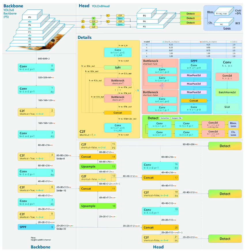
Diagram of YOLOv8’s architecture
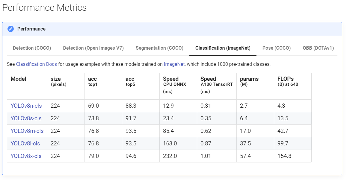
YOLOv8 is avaliable in many different sizes, as seen below. These offer a tradeoff between training time and overall accuracy.
Results
YOLOv8 Nano, 32 epochs
On our first attempt of running YOLOv8, we opted to use the smallest classification model (nano) and 32 epochs. While YOLOv8 is relatively plug-and-play thanks to it containing a pre-trained model, epochs are the main hyperparameter than needs tuning. The number of epochs is the number of times the training dataset is passed forward and backward through YOLO’s CNN. Too few epochs typically results in underfitting, while too many will result in overfitting.


- Accuracy: 94.375%
- f1-Measures: [0.8722, 0.9641] [healthy, diseased]
- Diagnostic Odds Ratio: 204.18
As proof of just how powerful YOLOv8 can be at classification out of the box, we immediately got strong results. Our accuracy was able to reach 94.375%, which beats out the accuracy of all our previous models. Still, there was a possibility our results could be improved on. The training loss and value losses hadn’t quite stabilized yet, indicating the possibility that further epochs might yield even better results.
YOLOv8 Nano, 100 epochs
For our second attempt of running YOLOv8, we opted to continue to use the smallest classification model (nano) but increase the overall number of epochs from 32 to 100.

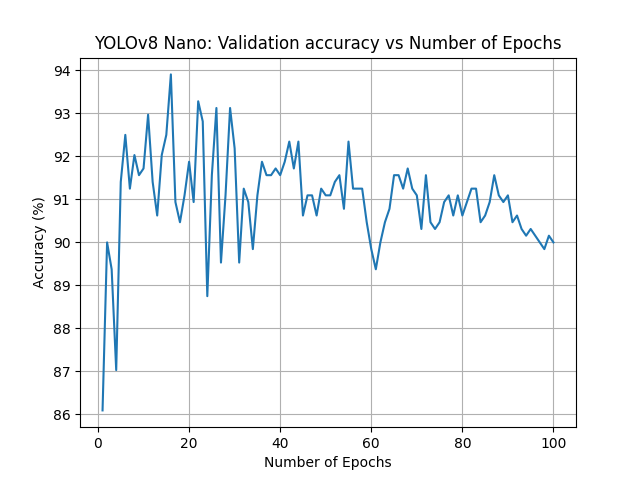

- Accuracy: 93.906%
- f1-Measures: [0.8612, 0.9609] [healthy, diseased]
- Diagnostic Odds Ratio: 171.83
Increasing the number of epochs weakened our results. While the best-case accuracy remained about the same at 93.906%, the model was clearly now overfitting. As the number of epochs increased pass 30, the accuracy gradually decreased. This told us that our initial guess of the number of epochs had been just about correct.
YOLOv8 Small, 32 epochs
For our third attempt of running YOLOv8, we opted to increase the size of our classification model to small but revert the overall number of epochs to 32.
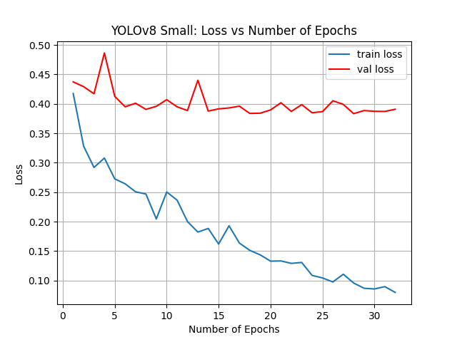
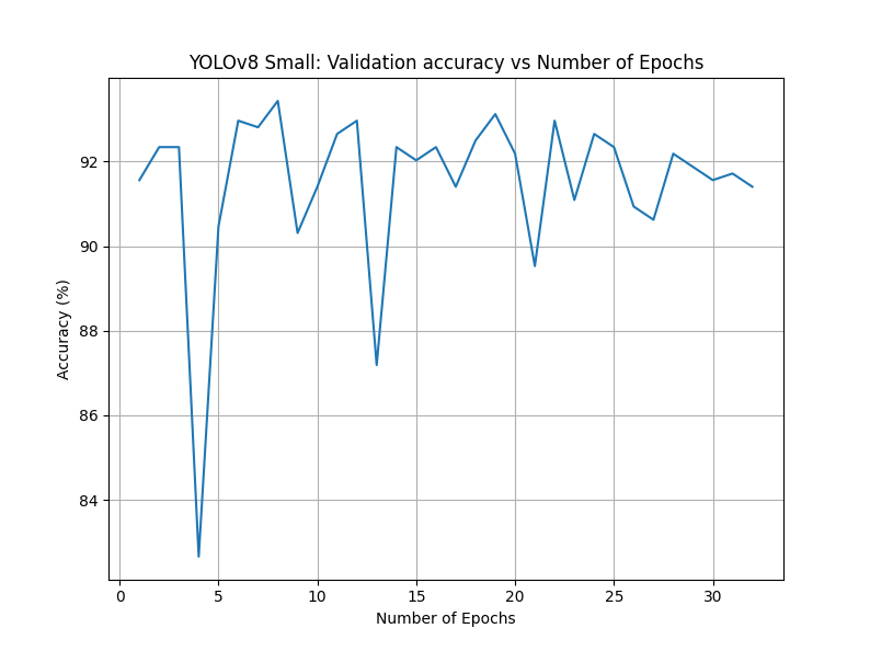
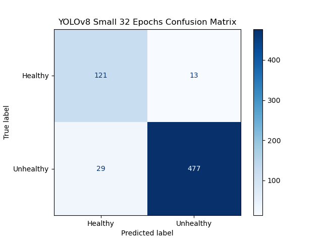
- Accuracy: 94.38%
- f1-Measures: [0.8521, 0.9578] [healthy, diseased]
- Diagnostic Odds Ratio: 153.09
Changing from nano to small had minimal effects on our overall accuracy. The best-case accuracy was now 94.38%, very similar to the original attempt. The graphs between this attempt and our third attempt were extremely similar as well.
Next Steps
Better YOLOv8 results are likely possible. While our tuning so far only yielded minimal results, it is likely our current hardware is a limiting factor that prevented us from pushing much further. Despite running YOLOv8 via local GPUs with CUDA, running larger models or more than 32 epochs took several hours. If we were to instead able to leverage a computing cluster, we could train using the large or XL versions of YOLOv8 to get even more accurate and consistent results.
Overall Results
For our results, we will only be comparing the most successful version of each model we discussed during the report (SVM, neural network, and YOLOv8). For SVM this was SVM with image processing, for our neural network this was CNN with Pytorch, and for YOLOv8 this was YOLOv8 nano with 32 epochs.
Visualizations
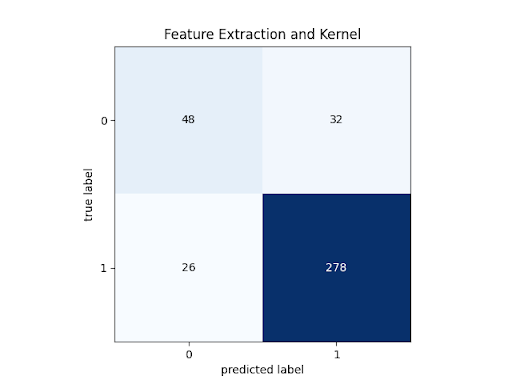
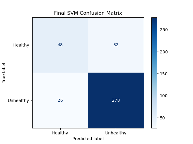
SVM Confusion Matrix:
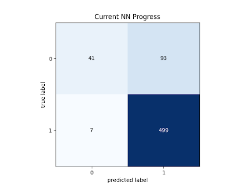
Neural Network Confusion Matrix:
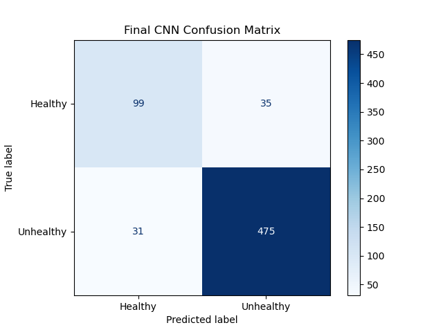
YOLOv8 Confusion Matrix:
Quantitative Metrics
SVM statistics:
- Accuracy: 84.90%
- f1-Measure: [0.6234, 0.9055] [healthy, diseased]
- Diagnostic Odds Ratio: 16.04
Neural net statistics:
- Accuracy: 89.69%
- f1-Measure: [0.7500, 0.9350]
- Diagnostic Odds Ratio: 43.34
YOLOv8 statistics:
- Accuracy: 94.375%
- f1-Measures: [0.8722, 0.9641]
- Diagnostic Odds Ratio: 204.18
Analysis of Models
SVM Analysis:
At a testing accuracy of 84.90%, this model reached our success target for accuracy. However, this does fall below our other measures.
Note that while the f1 score for the diseased eye classification (1) exceeds our stretch target, the f1 score for the healthy eye classification (0) falls well below our success target. This is visible on the confusion matrix: the first element on the diagonal has far lower relative accuracy (precision and recall) than the second element in the diagonal. This discrepancy is the reason the Diagnostic Odds Ratio is lower than our success target as well. Because the test returning a “healthy” verdict is not very informative, given that low relative performance, the total information of the test is much lower than desired.
Neural net statistics:
As expected, the CNN performed significantly better than the SVM.
At 89.69% accuracy, the CNN had almost 5% higher accuracy than the SVM, and almost reached our stretch goal of 90% accuracy. However, this model retained the same problem as the SVM, with low f1-score for healthy retinas. At 0.75, this is much closer to our success goal, but it is still an issue with the model. Additionally, this problem also still manifests in the Diagnostic Odds Ratio. 43.34 is much closer to our success target of 50, but still below it, because of the low degree of information gained by a healthy diagnosis.
YOLOv8 statistics:
Since, the YOLOv8 architecture is an incredibly sophisticated convolutional neural network which has been designed specifically for image classification, we expect this model to perform quite well, and it does.
At 94.38% accuracy, this model far exceeds our stretch goal for accuracy. Both classes have f1-scores above our success target, but even this model doesn’t reach the stretch goal for the healthy class, so maybe our stretch goal was a bit too much of a stretch. And finally, this classifier has a Diagnostic Odds Ratio of 204.18. This is far superior to our other models, especially since this model is so much better at discriminating the healthy eye cases, making it more diagnostically relevant.
Comparison of Models
While the performance of the SVM was very close to reaching success standards, and could possibly reach them with better feature engineering, it was far exceeded by the CNN, which was far exceeded by YOLOv8, as expected. The incredible performance of YOLOv8 on this dataset is a testament to transfer learning.
Next Steps
There are a number of steps that could be followed at this point in the project, however, some of them have requirements that we can not currently meet with the hardware we have. First of all, we would need more compute power for the CNN and YOLOv8 models. These models are already computationally expensive. If we wanted to try YOLOv8 Large, or expand our CNN, we would need far more computation power. That would also aid in cross-validation efforts. It was difficult to do rigorous cross-validation due to how expensive training our models was. Spending more compute-time to optimize hyperparameters may further improve performance. Additionally, our models were just binary classification. We could expand the models to accommodate multi-class classification or segmentation of troubling areas.
References
-
G. Lim, V. Bellemo, Y. Xie, X. Q. Lee, M. Y. T. Yip, and D. S. W. Ting, “Different fundus imaging modalities and technical factors in AI screening for diabetic retinopathy: A review,” Eye and Vision, vol. 7, no. 1, Apr. 2020, doi: https://doi.org/10.1186/s40662-020-00182-7.
-
L. Dong, Q. Yang, R. H. Zhang, and W. B. Wei, “Artificial intelligence for the detection of age-related macular degeneration in color fundus photographs: A systematic review and meta-analysis,” eClinicalMedicine, vol. 35, May 2021, doi: https://doi.org/10.1016/j.eclinm.2021.100875.
-
M. C. Viola Stella Mary, E. B. Rajsingh, and G. R. Naik, “Retinal fundus image analysis for diagnosis of glaucoma: A comprehensive survey,” IEEE Access, vol. 4, pp. 4327 - 4354, Jan. 2016, doi: https://doi.org/10.1109/access.2016.2596761.
-
https://scikit-learn.org/stable/modules/svm.html
-
https://scikit-image.org/docs/stable/auto_examples/features_detection/plot_hog.html
-
https://scikit-learn.org/stable/modules/generated/sklearn.neural_network.MLPClassifier.html
-
https://arxiv.org/abs/1506.02640v5
-
https://docs.ultralytics.com/models/yolov8/
-
https://pytorch.org/docs/stable/nn.html